Survey methodology
The American Trends Panel (ATP), created by Pew Research Center, is a nationally representative panel of randomly selected U.S. adults recruited from landline and cellphone random-digit-dial (RDD) surveys. Panelists participate via monthly self-administered web surveys. Panelists who do not have internet access are provided with a tablet and wireless internet connection. The panel is managed by GfK.
Data in this report are drawn from the panel wave conducted Feb. 26 to March 11, 2018, among 6,251 respondents. The margin of sampling error for the full sample of 6,251 respondents is plus or minus 1.9 percentage points.
Members of the ATP were recruited from several large, national landline and cellphone RDD surveys conducted in English and Spanish. At the end of each survey, respondents were invited to join the panel. The first group of panelists was recruited from the 2014 Political Polarization and Typology Survey, conducted Jan. 23 to March 16, 2014. Of the 10,013 adults interviewed, 9,809 were invited to take part in the panel and a total of 5,338 agreed to participate.6 The second group of panelists was recruited from the 2015 Pew Research Center Survey on Government, conducted Aug. 27 to Oct. 4, 2015. Of the 6,004 adults interviewed, all were invited to join the panel, and 2,976 agreed to participate.7 The third group of panelists was recruited from a survey conducted April 25 to June 4, 2017. Of the 5,012 adults interviewed in the survey or pretest, 3,905 were invited to take part in the panel and a total of 1,628 agreed to participate.8
A supplemental sample of respondents from GfK’s KnowledgePanel (KP) was included to ensure a sufficient number of interviews with adults in rural communities. The KP rural oversample was comprised of panelists in predefined rural ZIP codes. Rural ZIP codes were defined as those having 127 or fewer households per square mile.
The ATP data were weighted in a multistep process that begins with a base weight incorporating the respondents’ original survey selection probability and the fact that in 2014 some panelists were subsampled for invitation to the panel. Next, an adjustment was made for the fact that the propensity to join the panel and remain an active panelist varied across different groups in the sample. The final step in the weighting uses an iterative technique that aligns the sample to population benchmarks on a number of dimensions.
Gender, age, education, race, Hispanic origin and region parameters come from the U.S. Census Bureau’s 2016 American Community Survey. The county-level population density parameter (deciles) comes from the 2010 U.S. decennial census. The telephone service benchmark comes from the July-December 2016 National Health Interview Survey and is projected to 2017. The volunteerism benchmark comes from the 2015 Current Population Survey Volunteer Supplement. The party affiliation benchmark is the average of the three most recent Pew Research Center general public telephone surveys. The internet access benchmark comes from the 2017 ATP Panel Refresh Survey. Respondents who did not previously have internet access are treated as not having internet access for weighting purposes.
An additional raking parameter was added for Census Division by Metropolitan Status (living in a metropolitan statistical area or not) to adjust for the oversampling of rural households from KnowledgePanel. The Division by MSA benchmark comes from the U.S. Census Bureau’s 2016 American Community Survey. Sampling errors and statistical tests of significance take into account the effect of weighting. Interviews are conducted in both English and Spanish, but the Hispanic sample in the ATP is predominantly native born and English speaking.
The following table shows the unweighted sample sizes and the error attributable to sampling that would be expected at the 95% level of confidence for different groups in the survey:
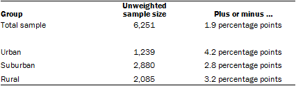
Sample sizes and sampling errors for other subgroups are available upon request.
In addition to sampling error, one should bear in mind that question wording and practical difficulties in conducting surveys can introduce error or bias into the findings of opinion polls.
The February 2018 wave had a response rate of 78% (6,251 responses among 7,996 individuals in the panel). Taking account of the combined, weighted response rate for the recruitment surveys (10.0%) and attrition from panel members who were removed at their request or for inactivity, the cumulative response rate for the wave is 2.2%.9
Secondary data sources and methodology
Most of the analysis in Chapter 1 and the secondary analysis in the overview is based on information collected in the 2000 decennial census and the 2012-2016 American Community Survey five-year file. The data are available on the Census Bureau’s American Factfinder web page.
The components of population change, natural increase and net migration are derived from the Census Bureau’s population estimates program. The analysis combines two separate series of population estimates. The 2000-2010 series comes from the Census Bureau’s 2010 vintage evaluation estimates, which was the last vintage to be based on the 2000 decennial census. The 2010-2014 series comes from Census’ 2017 vintage population estimates, which is based on the 2010 decennial census. Both series include an estimate of each respective county’s population on July 1, 2010. The historical trend was created by calculating the difference (either positive or negative) between these two estimates in each series and adding it to the residual change. After this correction, the 2014 population estimate equals the 2000 estimates base plus each year’s components of change for all counties. The 2014 population estimates were used in order to maximize comparability with the analysis based on the 2014 midpoint of the five-year American Community Survey file.
There are 3,142 counties and county equivalents in the U.S. We analyzed 3,130 individual counties or county groups, which encompass the entire U.S. resident population. We aggregated some individual counties into county groups in order to have geographic units that are consistent from 1990 to today. Since 1990, some states have changed their county boundaries. For example, in 2001 Colorado created Broomfield County from parts of four other counties: Adams, Boulder, Jefferson and Weld. In order to analyze the population change in these counties we examine the aggregate Broomfield group, which is the sum of the population of the five counties. Additional boundary changes occurred in Alaska and Virginia.
Counties are classified on the basis of the 2013 National Center for Health Statistics Urban-Rural Classification Scheme. In our analysis, a county’s classification does not change over time. Counties that were once non-metropolitan and were reclassified as metropolitan under subsequent U.S. Office of Management and Budget designations are considered to be metropolitan in all time periods in this report.
© Pew Research Center, 2018


